How to plot a 3D curve
Plotting a 3D curve consists of 3 steps:
-
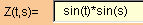
define the parametric expressions
of the curve for coordinates X, Y and Z by filling the appropriate fields
X(t,s),
Y(t,s) Z(t,s)
For
example 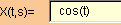
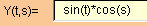
 For
example
For
example 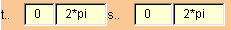
-
press the Plot-it! button

The 3D curve can then be navigated, modified,
and printed , moreover the plotting
settings and the visual settings can
be modified to adjust the curve rendering.
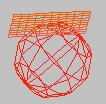
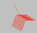
How to plot a tangent plane or
a normal vector of 3D curve in a fixed point
After have defined the parametric expressions
of the curve for coordinates X, Y and Z and defined the ranges
for parameters t and s it's possibile
plotting a tangent plane or a normal vector of 3D curve :
-
define a value, in the definition interval, for parameters
t and
s, in the fields named t =
and s=
For
example
-
press the Plot-Tg! button for plotting the tangent
plane
-
press the Plot-Nr! button for plotting the normal
vector
The 3D curve with its tangent plane or normal vector can then be navigated,
modified,
and printed , moreover the plotting
settings and the visual settings can
be modified to adjust the curve rendering.
Modifying a 3D curve
A 3D curve can be modified by changing its definitions in the X(t,s),
Y(t,s) Z(t,s) fields and/or the ranges
fields and plot-it again.
The modifications will no be visibible until the Plot-it! button is
pressed and the curve is plotted again.
If it is needed to modify the appearance of a given curve see navigating
the 3D curve, visual settings, plotting
settings.
Plotting Settings
The plotting settings contains parameters which regulate how the 3D curve
is computed and displayed.
In general a 3D curve is painted by rendering in 3D form a finite set
of points (sample points) calculated by using the definitions for
X(t,s), Y(t,s) and Z(t,s) and connecting the points with lines and/or surfaces.
The number of the point used for the plot (Grain and ranges)
and the way they are connected (Grid/not Grid) will result in a
different rendering for the same curve.
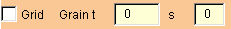
-
Grid parameter (default unchecked), if checked a grid it will be
drawn among the 3D curve computed points, otherwise lines are drawn.
-
Grain t/ Grain s parameters (default 0 means 20), for each parameter
(s or t) define the number of points in which the interval of the parameter
(as defined in ranges) is divided in order to compute. It is guaranteed
that the first and final point will coincide with the initial and final
points of the intervals. The default is 20 points both for t and s, that
result in 400 points to be calculated.
In general a greater value for grid parameters will result in a more defined
curve, but also in a greater computing time.
The above consideration is not completely valid with period functions
(such as sin or cos) where a great value for grain can result in unexpected
results.
Undefined Values/ Infinite Values
If the intervals for parameters contains values in which one of the parametric
function X(t,s)Y(t,s)Z(t,s) is undefined or it has infinite values,
this can or cannot be detected by Plot-it3D depending on the values of
parameters intervals and depending on the values of grain, which determine
the set of sample points used to compute the curve.
In the case that the set of sample points will include valuesfor which
functions X(t,s)Y(t,s)Z(t,s) are undefined or infinite value:
-
a function whose value is infinite or undefined will produce
the conventional value 0 (zero) and the event (infinite value/undefined
value) is signaled in the message bar.
Navigating the 3D curve
The 3D curve can be moved, zoomed,
rotated
and adapted by visual tools and visual settings
parameters.
The 3D curve can be rotated either by the Rotor panel buttons
or with the mouse cursor by drag&drop.
the Rotor panel contains buttons to rotate
the 3D Curve
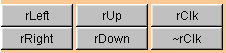
-
rLeft/rRight buttons rotate with respect to the vertical axes of
the screen
-
rUp/rDown buttons rotate with respect to the horizontal axes of
the screen
-
rClk/~rClk buttons rotate the curve Clockwise/CounterClockwise
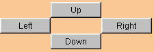
the Translate panel contains buttons to
move the 3D Curve in the indicated direction
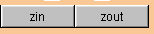
the Zoom buttons will respectively zoom the
figure in (zin) and out (zout)
the reset button will undo any translate
and rotate operation, but it will not affect zooming or other visual
settings

Visual Settings
Settings visual parameters will affect the current plotting and any further
plotting.
The effect of a change in a visual parameters is visible after
any action is made on the plotted image (i.e. clicking on the image or
zooming the image), it is not required to plot the image again after a
change on visual settings.

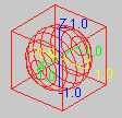
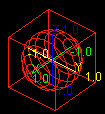
-
Axes (default checked), if Axes is checked , XYZ axes will
be drawn internally to the figure (respectively X
green,
Y yellow and Z
blue) and the extreme points of the axis will be labeled with the
minimum/maximum values which the functions assume on the axis. If Axes
is not checked no axes and no values are drawn.
-
Adapt (default not checked). If Adapt is not checked the
curve will appear in real proportion, that is to say that the figure is
downsized with the same proportional factor on the three axes to fit the
screen. In the case in which the range of min/max values has great differences
between two axis, the displayed figure will eventually reduce to a line
or to a point.In this case it prefereable to zoom in the figure or to use
the Adapt option. If Adapt is checked the curve will be drawn reducing
the proportion of each axis indipentently in order to fit the screen, and
to allow the maximum available space to each axis. In case of great difference
between the ranges of the axes this option can result in a better visualization
of the figure. It must be noted that since the reduction factor is independent
on each axes this can result in deforming figures such as spheres or perpendicular
lines.
-
Box (default checked). If Box is checked, a bounding box
will be drawn around the 3D curve.
-
Back (default not checked). If Back is checked, the 3D curve
is displayed on a black background, otherwise it is displayed on a grey
background
.
Printing a 3D curve
Currently only the browser default printing facilities is available, in
order to print the 3D curve with the web page containing the parameters:
choose
Print command on the File menu.
Since plot-it! will adapt to a variety of browser the result of printing
depends on the available version of the browser.
How evaluate
the coefficients of first and second fundamental form of 3D curve in a
fixed point
After having defined the parametric expressions
of the curve for coordinates X, Y and Z and defined the ranges
for parameters t and s it's possibile
evaluating the coefficients of first and second fundamental form of 3D
curve :
-
define a value, in the definition interval, for parameters
t and
s, in the fields named t = and s=
For
example
-
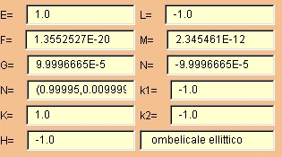
press the Form button for evaluating the factors
-
fields E=, F=, G= and L=,
M=, N= will repsectively show the values of coefficients of
first and second fundamental form;
-
field N= shows the values of components of
the normal vector;
-
fields k1=, k2= shows the values of the main
curvatures
-
fields K=, H= shows the values of the Gaussian
curvature and Mean curvature
Expressions
A valid Plot-it! expression is any expression built by parameters
t and s, numerical
constants, predefined constant symbols,
operators
and functions.
Invalid expressions can cause no effects on the plotting or unpredictable
results.
Parameters
parameters t and s
can be specified inside any function expression,
values will be assigned to the parameters for evaluating functions,
depending on the specificied ranges and settings
Ranges
Parameters ranges, represent the interval of values which are used
to evaluate the target functions.
min, max values are specified inserting the appropriate fields
constant expressions, i.e. expressions cointaining either numerical
constants o special constant symbols,
but no parameters.
A range is valid if the values are not empty and min <= max.
If a value is omitted and/or the interval is invalid the result is
unpredictable.
An invalid range is signaled in the message bar.
Example of valid [min,max] ranges specifications are:
[-1,1] [0,1000] [0, 2*pi] [log(10),1-pi/2,]
Constants
Two type of constants are allowed in Plot-it expressions: numerical
constants and special constants.
Numerical Constant
Plot-it accepts in input numerical constants in standard notation:
-
standard notation with/without sign and decimal point
Example: 2345
0
3.1002 150000
-
scientific notation is used for output of very large/small
numbers:
Example: -9.03342e+021
1.3653e-012
Special Constants
Predefined special constants are available in order to enhance the numerical
precision of computations and improving clarity of expressions:
-
e = 2.7182
constant basis for exponential and logarithm functions
-
pi = 3.1415
trigonometric constant
Operators
Conventional arithmetical operators and additional math
functions can be used in Plot-it expressions:
-
unary minus sign <expr> Es. (234) is equivalent to 234
-
+ sum <expr>+<expr> Es. 3 + 12
-
minus <expr><expr> Es. 3 12
-
* multiplication <expr>*<expr> Es. 3 * 12
-
/ division <expr>/<expr> Es. 3 / 12
-
^ power operator <expr1>^<expr2> , <expr1> is the basis and
<expr2> is the exponent Es. 3^2 that is 9.
-
( ) parentheses, alterate standard precedence rules Es. (3 12)* 4
/ (2 / 3)
Functions
Several mathematical functions are available in Plot-it!.
Functions calls in expressions are specified in usual prefix notation
fun(arg1,
,argn)
where fun is the function name and arg1,
,argn are the function
arguments separated by comma.
Function arguments, can recursively contains expressions and functions
as in sqrt(2-sin(s*e))
Basic Functions
-
abs(<arg>) absolute value of <arg>
-
sqrt(<arg>) square root of <arg>
-
exp(<arg>) exponential function,
constant e raised to the power of <arg>
-
log(<arg>) logarithm of <arg>
to the base e
Trigonometric
functions
-
sin(<arg>) sine of <arg>
-
cos(<arg>) cosine of <arg>
-
asin(<arg>) inverse sine of <arg>
-
acos(<arg>) inverse cosine of <arg>
-
tan(<arg>) tangent of <arg>
-
cot(<arg>) cotangent of <arg>
-
atan(<arg>) inverse tangent of <arg>
-
acot(<arg>) inverse cotangent of
<arg>
-
sinh(<arg>) hyperbolic sine of <arg>
-
cosh(<arg>) hyperbolic cosine of
<arg>
-
tanh(<arg>) hyperbolic tangent of
<arg>
-
asinh(<arg>) inverse hyperbolic
sine of <arg>
-
acosh(<arg>) inverse hyperbolic
cosine of <arg>
-
atanh(<arg>) inverse hyperbolic
tangent of <arg>
Il presente software plot-it!, plot-it!3d, plot-it!2d,
i sorgenti, le relative classi java, e pagine html sono di esclusiva
proprietà degli autori,
qualsiasi utilizzo per fini commerciali è escluso.